
Lesson 5-5
Item cost dynamic analysis
As we discussed earlier in this Lesson, the Material item’s cost going up means that we need to increase the selling price. Otherwise, our profit goes down. And other way round - when the Material item’s cost goes down our profit goes up. So, the dynamic of item cost changes means a lot for making the right calls in everyday life of our small enterprise.
Therefore, the director of Handy Guys LLC set the task to implement a new functionality - get a daily item cost dynamic report on all Materials.
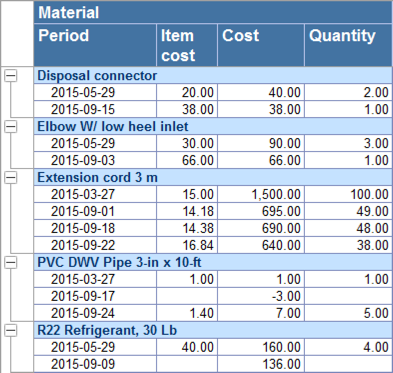
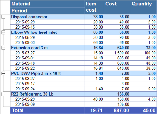
We already have an accumulation register storing the data we need - MaterialCost. It has two resources - Quantity and Cost, so, if we get the resources’ balances for any given day and then divide the Cost by the Quantity we will get the ItemCost for this day. The resulting table we get should look like this.
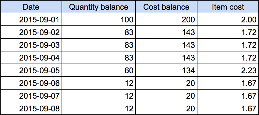
The table contains a daily history of Material item cost changes. Item cost column is calculated as Cost balance / Quantity balance. Note that some days contain no selling or buying the Material, and, therefore, there are no balances or item cost changes at these points. On the other hand, some days can contain more than one operation with this Material. In this case, the overall balance change will include all of them summed up.
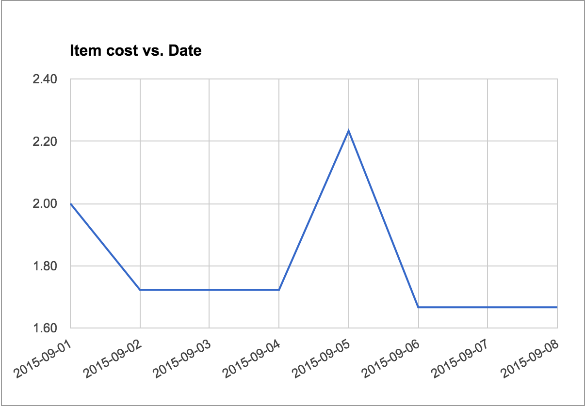
Besides of seeing the data in the form of a table, we could use the diagram view of them.
Let’s start with the table and look how we can get it.
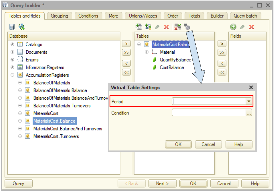
We already know how to use the accumulation register balance table, but it’s hardly a good choice for this specific task. If you run the Query Builder and open MaterialsCostBalance table parameters you will see that we can specify the only date parameter, so we need to query the table in a cycle passing the dates one by one (which is a pretty bad idea performance-wise).
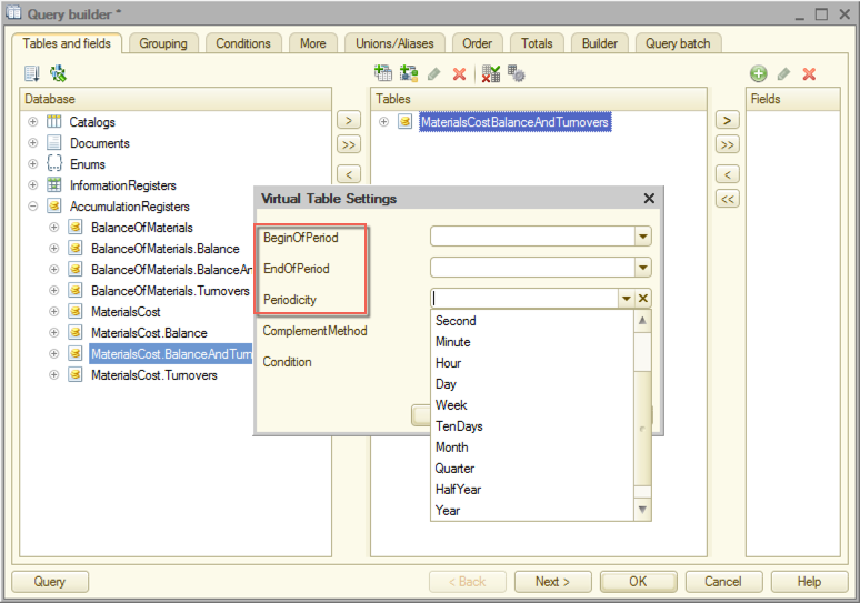
Let’s see what other MaterialsCost-related tables we have in the Query Builder list.
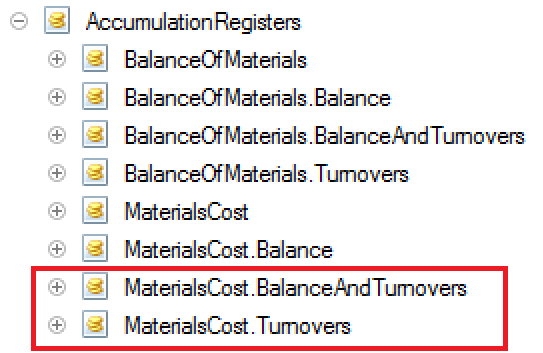
Both tables’ parameters look like we can get all we need from them. We see the period boundaries settings and the periodicity parameter that can be set to anything from Second to Year.
To get a better idea of what’s inside of the BalanceAndTurnovers virtual table, let’s build a simple report on its content.
BalanceAndTurnovers virtual table. Plain list report.
OK, now let’s see the content of the BalanceAndTurnovers virtual table.
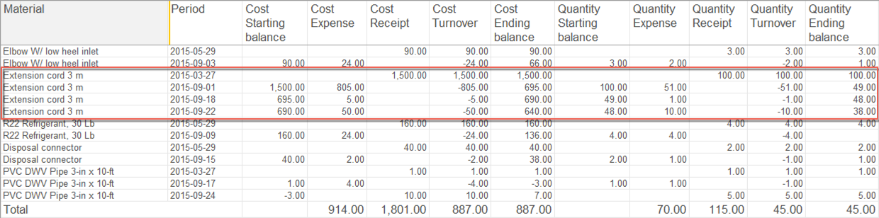
The highlighted part reflects the daily history of the Extension cord buying and selling. The first line shows the initial state and the first operation. Cost and Quantity starting balances are equal to zero. Nothing to expense so far, so there are no expenses, but there is the receipt of 100 cords for a total amount of $1,500. These two numbers are shown in the Quantity receipt and Cost receipt columns correspondingly.
The turnover calculation formula is Sum(Receipts) - Sum(Expenses). In other words, turnover reflects the overall change in the balance during the given period of time (day in our case). We had some resource balance at the beginning of the period, then we added some more (bought more material) and subtracted some (sell material). The result is the ending balance for this period. So, this is two main formulas explaining the turnover term, and it’s connection to starting and ending balances.
Turnover = Sum(Receipts) - Sum(Expenses)
Ending balance = Starting balance + Turnover
Therefore, the first line (2015-03-27) cost turnover is 1,500 (= 1,500 - 0) and the ending balance for that day is 1,500 (= 0 + 1,500). The first line quantity turnover is 100 (= 100 - 0) and the ending balance is 100 (= 0 + 100).
Next important (and pretty simple) formula is the following:
Ending balance(last period) = Starting balance(current period)
Therefore, the second line (2015-09-01) starting balances are equal to the first line ending balances. This day 51 cords were sold for the total amount of $805, so the cost ending balance is 695 (1,500 - 805) and the quantity ending balance is 49 (100 - 51).
Getting back to our task (trace the dynamic of materials items’ cost): looks like we have all we need in the BalanceAndTurnovers table, so let’s tidy up the table and use it as a part of the report we need.
Here is a list of things I want us to correct in the current report:
- Visually separate different materials from each other;
- Correct the period column: get rid of the time and change the date format to YYYY-MM-DD;
- Exclude the starting balance, expense, receipt and turnover columns. Rename the Ending balance columns into Cost and Quantity correspondingly;
- Add a new column Item Cost = Cost / Quantity.
Tidying the report
So, this is the report we’ve got for now.
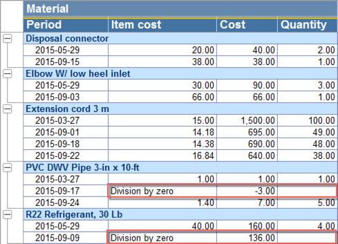
The obvious reason behind this “Division by zero” error message is that we had no material left at these moments, so the Item Cost cannot be calculated. Let’s decide that in this case we will output 0. But how can we do that?
OK, here is the thing. This expression we used to calculate the ItemCost field value, obviously contains the string expression interpreted by the report builder. We used fields names and the division operation there but what is the complete syntax of this expression language?
If you look at the 1C:Enterprise 8.3 Developer Guide you will find the chapter - 10.3.4. Data composition system expression language - containing the references we need. The operator we can use for our purposes is CASE.
This is how it works.
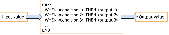
Basically, choice checks the input value against the set of conditions and return an output value specified in the first condition that is true. In our case we could use the following expression:
CASE
	WHEN QuantityClosingBalance  0 THEN CostClosingBalance / QuantityClosingBalance
	ELSE 0
END
After this correction, the report looks like this.
Resources in DCS
If we contract all first level nodes of the tree, the report becomes completely uninformative.
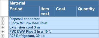
We can see the Materials’ names but nothing else. Let’s make this view more useful for a user. Would be great, for example, to show the current (last known) values of all the fields here. But how can we do that?
These group values cannot be obtained from the data set we use (it contains only detailed records), but we can ask the DCS to calculate it. In order to do so we need to declare them as resources and specify the calculation expressions. Resources - is numeric fields that can be used by DCS to calculate aggregated values when grouping the primary data retrieved from the data set.
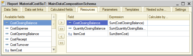
So, let’s open the DCS and go to the Resources tab. There we need to drag and drop the necessary fields to the right side of the form telling the DCS to treat them as resources. The DCS automatically specifies a calculation expression as Sum().
At the first glance, this is not what we need (we want the last known value - not the sum of all values) but let’s give it a try and look at the resulting report.
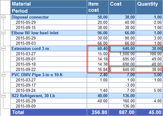
Surprisingly, the Cost and the Quantity totals show exactly what we need - the last known value in spite of the fact that we used Sum aggregate function. On the other hand, the Item Cost Total shows the sum of the detailed records, which is not what we need but it, at least, conforms with the calculation formula. OK, how does it work at all?
Here is a thing. Any data set field can belong to a so-called Role (not to be confused with the application Roles defining the access rights). The DCS field Role defines the way this field is to be treated by the DCS processor. The DCS automatically recognizes the fields you retrieve from the Data Set and specifies their Roles (if the Autofill checkbox is selected).
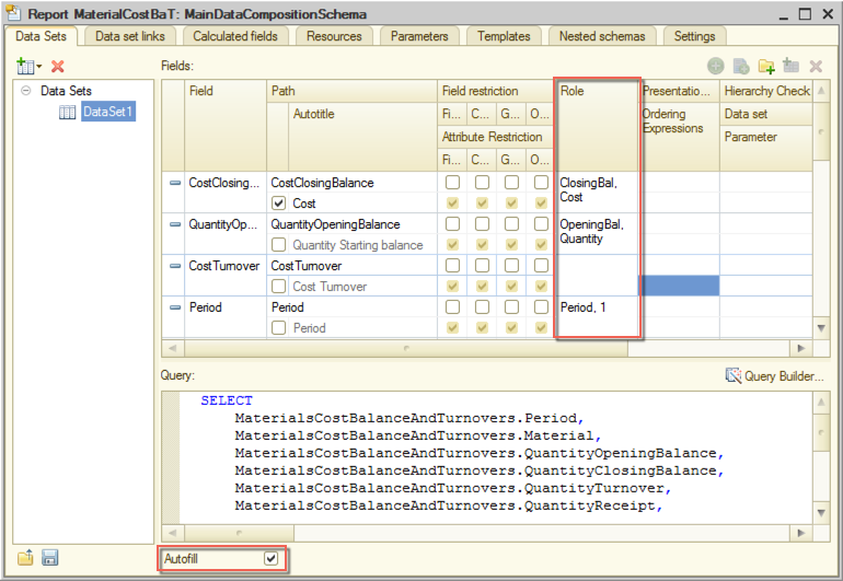
The Cost and Quantity Closing Balance fields have a Role “Balance” and the balance type “Closing balance”.
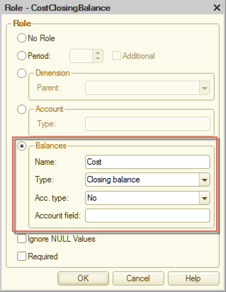
This gives DCS a hint of the nature of the data these fields contain. This is how the DCS knows that it should take the last known detailed records value rather than sum them up. In other words, Sum operator gives you the bottom-line value, which can be a sum or the last known value of the subordinate records depending on the field’s role.
So, we leave the CostClosingBalance and QuantityClosingBalance resources expressions as they are.
Now, to ItemCost recourse expression.We definitely don’t need to sum up the subordinate records here. What we need is Sum(CostClosingBalance) / Sum(QuantityClosingBalance). Sum operators give us the last known values, we divide one by another and get the last known value of the item cost. Besides that, we need to take into account the “Division by zero” problem we discussed earlier. So the final expression for the ItemCost resource will be the following.
CASE
	WHEN Sum(QuantityClosingBalance)  0
THEN Sum(CostClosingBalance) / Sum(QuantityClosingBalance)
	ELSE 0
END
We also need to specify the ItemCost calculated field type (Number(15, 2)) to fix the formatting problem.
The resulting report looks like this:
Now let’s make it more intuitively obvious by representing the same data in a form of a diagram. It would also help if we allow a user to specify the period of time he wants to see the data for.
Adding a diagram to the report
Now we have the report with a table and diagram showing the history of Item Cost changes for all Materials we have.
Lesson 5-4 | Course description