Lesson 13. Reports

Estimated duration of the lesson is 4 hours 30 minutes.

Since the overall duration of the lesson is quite long, you can go through the lesson in parts and make interruptions after each of the six reports developed during the lesson.

CONTENT:

Theory.

Ways to Access Data.
Working with Queries.

Sources of Query Data.
The Query Language.

Data Composition System.

Selecting Data from One Table.
Selecting Data from Two Tables.
Display of Data for All the Days in the Selected Period.
Getting Current Values from a Periodic Information Register.
Using Calculated Fields in a Report.
Data Output to a Table.
Theory. Virtual Query Tables.
Quiz.

Now it is time to get to know one of the important tools of the 1C:Enterprise platform - the data composition system. During this lesson we will discuss design of several reports that will be used in our configuration. We will use these reports as an example to explain main features of the data composition system.

As a rule, every report involves obtaining a complex selection of data that is grouped and sorted in a specified manner. Data composition system is a powerful and flexible tool that makes it possible to carry out all the required actions: from obtaining data from various sources to displaying the data in a user-friendly manner.

Most frequently the initial data required for a report are located in the database. 1C:Enterprise 8 query language is used to specify the information and its sources for the data composition system.

On the report designing step you can define default report settings for the user to be able to run the report for execution right away. At the same time a user can also change report settings manually and execute the report. At that the data composition system will generate another query and will present final data otherwise, i.e. in compliance with the user-specified settings.

In the beginning of the lesson we will discuss general information about the 1C:Enterprise query language and the data composition system.

Next we will use the examples of creating specific reports to understand how data composition system should be used for practical tasks.

Theory

Ways to Access Data

1C:Enterprise 8 supports two methods for accessing data stored in a database:

• Object (for reading and writing);
• Table (for reading).

The object method of accessing data is implemented using 1C:Enterprise script entities.

We have encountered some of the entities during the previous lessons.

An important feature of object data access method is that when we call for a 1C:Enterprise script entity, we call for some data set available in the database as a whole.

For example, the object DocumentObject.ServicesRendered will contain values for all the Services Rendered document's attributes and all the tabular sections it contains.

The object technique provides for maintenance of object integrity, object caching, calls to the appropriate event handlers, etc.

Table access to data in 1C:Enterprise 8 is implemented using database queries that are written using query language.

This technique allows a developer to work with separate fields in database tables containing some data.

The table method is used to get information from a database based on certain conditions (filter, grouping, sorting, merger of multiple selections, calculation of totals, etc.). The table technique is specially designed to handle large volumes of data which are stored in a database, and for obtaining data that matches specified criteria.

Working with Queries

Working with queries involves use of the 1C:Enterprise script entity named Query. It allows us to obtain information from database fields in the form of selections, based on the rules we specify.

Sources of Query Data

Queries obtain their source information from a set of tables. These tables provide a developer with data from actual database tables in a form that is convenient for analysis.

All the tables used by the query language can be joined into two large groups: actual tables and virtual tables (fig. 13.1).

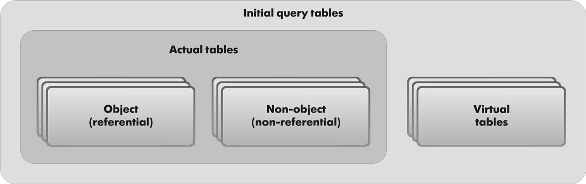
Fig. 13.1. Query Tables

You can view the assortment of tables available for a query along with their descriptions in the Syntax Assistant (section Working with Queries4Query Tables).

Actual tables are distinguished by the fact that they contain data from one actual table stored in the database.

For example, Catalog.Clients is an actual table that corresponds to the Clients catalog same as the AccumulationRegister.BalanceOfMaterials table that corresponds to the BalanceOfMaterials accumulation register.

Virtual tables are usually generated based on data drawn from multiple database tables.

For example, AccumulationRegister.BalanceOfMaterials.BalanceAndTurnovers is a virtual table that has been generated based on multiple tables of the BalanceOfMaterials register.

In some cases, virtual tables can also be generated based on a single actual table (for example, the virtual table Prices.SliceLast is generated based on the table of the Prices information register).

However, all the virtual tables share one thing in common: they can be assigned a number of parameters that will define the data to be included in such tables. The assortment of parameters may vary for different virtual tables and is defined by the data stored in the source database tables.

There are two types of actual tables: object (referential) and non-object (non-referential).

Referential type data is stored in object (referential) tables (catalogs, documents, chart of characteristic types, etc.). Whereas non-object (non-referential) tables store all the other types of data (constants, registers, etc.).

The distinctive feature of object (referential) tables is the fact that they contain a Reference field, which links to the current record. User object presentation can be obtained for such tables as well. These tables can be hierarchical tables. Fields of such tables may include nested tables (tabular sections).

The Query Language

The algorithm that will be used to select data from the query source tables is defined using dedicated query language.

A query text may consist of several parts:

• query definition;
• query union;
• result ordering;
• autoorder;
• definition of totals.

The only mandatory part of the query is the first one - the query definition. All the others are included as required.

A query definition specifies data sources, selection fields, grouping, etc.

Query union describes how the results of several queries are to be merged.

Result ordering describes the criteria for ordering rows within the query results.

AutoOrder allows you to enable automatic ordering of rows in a query result.

Definition of totals describes what totals are to be calculated in the query and how the results should be grouped.

Note that when query language is used to describe data sources in the data composition system, the definition of totals section of the query language is not used. This is due to the fact that data composition system calculates totals itself based on the settings implemented by the developer or the user.

Use of various syntax structures of the query language is described in details in the built-in help opened in the Designer mode: Help > Help Contents > 1C:Enterprise > 1C:Enterprise Script > Working with Queries, as well as in the manual "1C:Enterprise 8.2. Developer Guide," chapter 8 "Working with Queries".

We will discuss query language in more details later when we create specific reports.

We will not create any queries manually. For the majority of reports developed using data composition system, a query can be created using queries wizard.

So our goal by the end of this lesson is to learn how to read and understand the code of such queries to be able to edit them in the future.

Data Composition System

Data composition system is intended to create arbitrary reports in the 1C:Enterprise and includes multiple major parts.

Data composition schema includes initial data for report composition, i.e. data sets and methods of working with them (fig. 13.2).

Fig. 13.2. General flowchart for data composition system

A developer creates data composition system where they describe query text, data sets, connections between them, available fields, data access parameters and also define initial composition settings, i.e. report structure, data appearance template, etc.

For example, a composition schema may include a data set as follows (fig. 13.3).

On the figure above you see the data composition schema wizard window that includes data source, query text and the fields selected by the query.

A report of the data composition system a user will get is not simply a table of records that satisfy the conditions of the query.

A composition system report has a complex hierarchical structure and may include multiple items, such as groupings, tables, and charts.

A user may edit an existing report structure or create an entirely new report structure. A user may also customize a required selection, appearance of report structure items, obtain details for every item, etc.

For example, the following report structure including one table and one chart may be specified (fig. 13.4).

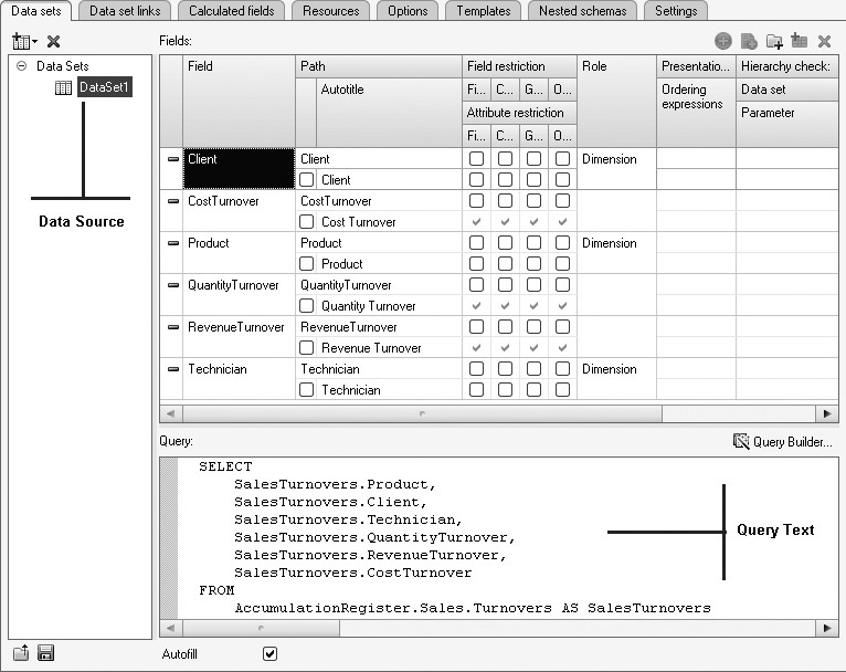
Fig. 13.3. Sample composition schema (data set and query using this set)

Fig. 13.4. Possible report structure

In this case the generated report will look as follows (fig. 13.5).

In the report above the table will consist of the records of SalesTurnover accumulation register related to the clients and services provided to such clients. These records are joined into groups by the technicians who performed the requests. And a grouping will display the list of services provided by this technician and the materials used in the process.

As we have already mentioned early in this section, data composition system is an aggregate of multiple objects. When a report is generated and executed, data is transferred in sequence from one object of the data composition system to another object until the final result is obtained, i.e. the document displayed to the user.

The algorithm of interactions between such objects is as follows:

• A developer creates data composition schema and default settings. Usually a large number of various reports may be created based on one data composition schema. Data composition settings (either created by a developer or modified by a user) define the specific report that will be generated.
• Based on the composition schema and available settings the template compiler creates a template. This is the stage of preparation to report execution. Data composition template is a finished assignment for composition execution by the processor. This template includes the required queries, templates of report areas, etc.
• Data composition processor selects data from the infobase based on the composition template, aggregates and arranges the data.
• Composition result is processed by the output processor so that the user finally receives the resulting spreadsheet document.

This sequence of operations can be presented as a flowchart as follows (fig. 13.6):

Fig. 13.6. Flowchart of composition system operations

Selecting Data from One Table

Let us create a report named Services Rendered Documents Register using the data composition system.

Using this report as an example we will demonstrate how data can be selected from one database table and how such data should be output in a specific order. We will also learn how to use details in a ready report.

This report will print out a list of the ServicesRendered documents from the database, sorted by their date and number (fig. 13.7).

Fig. 13.7 Report Results

In the Designer Mode

In the Designer add a new Report configuration object. Repeat the first steps involved in report creation discussed in the lesson 6.

On the Main tab enter ServicesRenderedDocumentsRegister as the name of the report.

Enter List of Rendering Services as the Extended presentation for how the report will appear in the software interface.

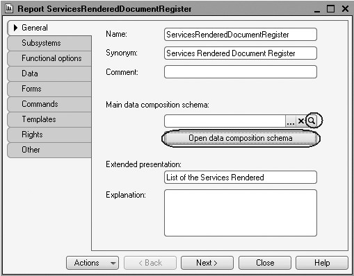
Fig. 13.8 Main Report Properties

Create data composition schema for the report. To do so, click Open Data Composition Schema or the opening button marked with a magnifying glass (fig. 13.8).

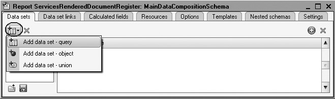
Click Finish in the dialog window of the template wizard. In the data composition schema wizard create Data Set - Query (fig. 13.9).

A Query for a Data Set

Click the Query Wizard button to launch the query wizard.

For the data source of the query select the object (referential) table

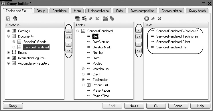
Fig. 13.10. Selected fields for a query

Select the following fields from this table (fig. 13.10):

• Warehouse;
• Technician;
• Client;
• Reference.

NOTE

You can move the highlighted items between lists by dragging and dropping them or by double-clicking them. Or you can use the buttons , , , .

Field Aliases

Go to the Unions/Aliases tab and specify that the Reference field will have an alias of Document (fig. 13.11).

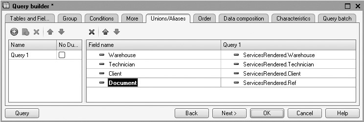
Fig. 13.11. Defining aliases for query fields

TIP

It is better to change field names in the query because in this case they will be transferred to the data composition schema into three columns right away: Field, Path, and Title, so you will not have to modify them additionally.

Records Order

Now go to the Order tab and specify that the query result should be ordered by the value of the Document field (fig. 13.12).

Analysis of the Query Text

Click OK and review the query generated by the query wizard (listing 13.1).

Listing 13.1. Query Text

SELECT
	ServicesRendered.Warehouse,
	ServicesRendered.Technician,
	ServicesRendered.Client,
	ServicesRendered.Ref AS Document
FROM
	Document.ServicesRendered AS ServicesRendered
ORDER BY Document

As we have mentioned above, query text begins with the query definition section (listing 13.2).

Listing 13.2. Query Description

SELECT
	ServicesRendered.Warehouse,
	ServicesRendered.Technician,
	ServicesRendered.Client,
	ServicesRendered.Ref AS Document
FROM
	Document.ServicesRendered AS ServicesRendered

The query definition begins with the required SELECT keyword.

The next section is a list of selection fields. This list describes the fields that should be included in the query result. The list can contain the fields themselves as well as certain expressions calculated based on the values in the fields.

The data sources are specified after the keyword FROM. Sources are the source query tables, the contents of which will be processed in the query.

In this case this is the object (referential) table Document.ServicesRendered. Aliases of the source data are specified after the keyword AS.

In our case, it is ServicesRendered. Thereafter, the query text can reference that data source using an alias.

We see such a reference in the list of selection fields (listing 13.3).

Listing 13.3. Selection Fields Definition

SELECT
	ServicesRendered.Warehouse,
	ServicesRendered.Technician,
	ServicesRendered.Client,
	ServicesRendered.Ref AS Document
FROM
	Document.ServicesRendered AS ServicesRendered

Selection fields may also have aliases which can be used to address these fields in the query text in the future. In our situation the alias is Document for the Reference field.

After the query definition section, our example continues with result ordering section (listing 13.4).

Listing 13.4. Query result ordering

ORDER BY
	Document

The ORDER BY clause allows you to sort rows in the query result. Following this keyword clause, we enter order criteria that will generally be an enumeration of fields (expressions) and sort order.

In our situation the result will be ordered by the Document field (which is also the ServicesRendered.Ref field). The result will be sorted in ascending order (if sorting order is not specified explicitly, sorting in ascending order is applied).

Now we will complete the discussion of the query text and proceed to settings of the data composition schema.

Settings

Go to the Settings tab and create default settings that define how information is displayed in a report.

Hierarchical report structure may include various combinations of three key items:

• Grouping - to display information as a regular linear report.
• Table - to display information as a table.
• Chart - to display information as a chart.

To add a new item (grouping in our case), highlight the Report root item in the report structure tree and open its context menu.

Alternatively you can click Add in the command bar of the window or press Ins (fig. 13.13).

Fig. 13.13. Adding a new grouping to a report

In the grouping selection window simply click OK (in doing so we specify that the grouping will display detailed records from the infobase).

The report structure will have a grouping named Detailed records.

On the Selected fields tab drag the fields to be included in the report from the list of available fields:

• Document;
• Warehouse;
• Technician;
• Client.

NOTE

You can add the available fields to the list of selected fields by dragging and dropping them; by double-clicking available fields; or by clicking Add to the right of the list of selected fields. You can reorder the selected fields later using Up and Down buttons or by dragging and dropping them.

This will result in the following arrangement of the report settings window (fig. 13.14).

This completes creating the report.

Finally, we will define the subsystems where our report will be displayed.

Close the data composition schema wizard and in the editor of the ServicesRenderedDocumentsRegister Report configuration object navigate to the Subsystems tab.

Check Rendering Services subsystem in the list.

So a link to our report will be automatically added to the action panel of this subsystem (fig. 13.15).

Fig. 13.15. Defining a list of subsystems where a report will be displayed

In the 1C:Enterprise Mode

Launch 1C:Enterprise in the debugging mode and see how the report works.

In the 1C:Enterprise window that opens you see that the action panel of the Rendering Services section now has a command to execute the report named Services Rendered Documents Register in the group of commands for reports execution.

Note that on mouse-over a tooltip appears with the text List of Services Rendered (defined in the Extended Presentation property we have defined for the report).

Execute this command (fig. 13.16).

This will open an automatically generated report form.

Note that the title of this form also has List of Services Rendered (because it is also defined by the Extended presentation property).

Click Generate (fig. 13.17).

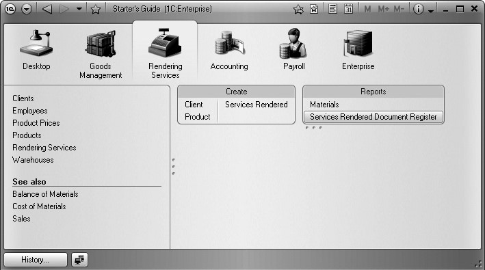
Fig. 13.16. Command to generate a report

You see that the report contains the register of Services Rendered documents.

If you double-click the Document field, you can open the source document and execute other actions to obtain details that are available in the data composition system.

The example of this report demonstrates how to use the data composition schema wizard and gives you an idea of several basic query language statements.

Selecting Data from Two Tables

The Service Evaluation report will contain information about which services were most profitable for Jack of All Trades within a given period (fig. 13.18).

Using the Service Evaluation report as an example we will demonstrate how to select data for a given period, how to set query parameters, how to use data from multiple tables in a query, and how to include all the data from one of the sources into the query result.

We will also get to know how to work with data composition system parameters, how to use default dates and will also familiarize ourselves with quick custom report settings.

Besides, we will learn to customize filter and conditional appearance further in the reports.

In the Designer Mode

Add a new Report configuration object.

Enter ServiceEvaluation for the report name and run the data composition schema wizard.

Add a new Data Set - Query and open the query wizard.

Query for a Data Set

Left Join of Two Tables

As a data source for the query we will select an object (referential) table Products and a virtual table of the Sales.Turnover accumulation register.

In order to avoid ambiguous names in the query, we will rename the Products table to ProductsCat.

To do so, highlight it in the Tables list, open its context menu and select Rename Table (fig. 13.19).

We will move the following fields from these tables to the list of fields:

ProductsCat.Ref and SalesTurnover.SalesRevenue (fig. 13.20).

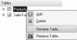
Fig. 13.19. Renaming a table

Fig. 13.20. Selected fields in the query

Switch to the Links tab.

Since multiple tables participate in the query now, you should determine relations between them.

By default the platform will create a link using the Product field. This means that the value of the Product dimension of the Sales register should match the link to the item of the Products catalog.

But we need to clear All for the SalesTurnover table and check it for the ProductsCat table.

This is how we select Left Join as the link type, i.e. the result of the query will include all the records of the Products catalog and those records of the Sales register that meet the link criterion for the Product field.

That way, the query results will contain all the services, and sales revenue will be indicated for some of them. No value will be displayed for those services that were not rendered within the selected period.

The following example can be used to visually describe the relation between the two tables described above (fig. 13.21).

Fig. 13.21. Links of records in query tables

After the actions above the Links tab will look as follows (fig. 13.22):

Fig. 13.22. Defining relations between tables

Record Filter Condition

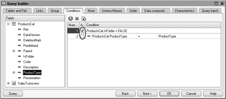
Now go to the Conditions tab and define a filter for the folders of the Products catalog not to be included into the report.

To do so, expand the ProductsCat table, drag the field IsFolder to the list of conditions, check Arbitrary and enter the following text to the Condition field (listing 13.5).

Listing 13.5. Query Condition

ProductsCat.IsFolder = FALSE

This is how we specify that only those records of the Products catalog should be selected that are not folders.

The operation of this condition can be visually described using the following example. On the left you see the source table of the Products catalog while on the right you see the records that will be selected from this table. (fig. 13.23).

Fig. 13.23. Filtering product records in a query

The second condition is that selected items must be services. This is a Simple Condition. To create the condition, drag the ProductType field to the list of conditions.

The platform will automatically create a condition which defines that the type of product should match the value of the ProductType parameter.

In the future prior to execution of the query, we will transfer the enumeration value Service to the ProductType parameter.

Operation of this condition can also be visually described using the following example. On the left you see the records of the Products catalog filtered out using the first condition. Located on the right are only the records that are services (fig. 13.24).

Fig. 13.24. Filtering product records in a query

This will result in the following appearance of the Conditions tab (fig. 13.25).

TIP

Filters can be used both in the query itself and in the report settings. This is true both for sorting and grouping. It is better to use a filter in the query if the records that do not meet the query condition will definitely not be needed in the report. Sorting and grouping should better be used in the report settings to make the report more flexible.

Field Aliases

Go to the Unions/Aliases tab and indicate that the catalog item (Ref field) will be represented by the alias Service, while the register field will have the alias Revenue (fig. 13.26).

Fig. 13.26. Defining aliases for query fields

Records Order

Switch to the Order tab and indicate that query results are to be sorted by the Revenue field in descending order (fig. 13.27).

Now we are done creating the query. Click OK. Return to the data composition schema wizard.

Analysis of Query Text

The text of query generated by the platform will look as follows (listing 13.6).

Listing 13.6. Query Text

SELECT
    ProductsCat.Ref AS Service,
    SalesTurnovers.RevenueTurnover AS Revenue
  FROM
    Catalog.Products AS ProductsCat
      LEFT JOIN AccumulationRegister.Sales.Turnovers AS SalesTurnovers
      ON (SalesTurnovers.Product = ProductsCat.Ref)
  WHERE 
    ProductsCat.IsFolder = FALSE
    AND ProductsCat.ProductType = &ProductType
  ORDER BY
	Revenue
  DESC

First we have the usual query definition section, this time containing statements we have not encountered before.

In defining the query sources (after the keyword FROM) we used the option of declaring multiple data sources (listing 13.7).

Listing 13.7. Defining Multiple Query Sources

  FROM 
    Catalog.Products AS ProductsCat 
      LEFT JOIN AccumulationRegister.Sales.Turnovers AS SalesTurnovers 
      ON (SalesTurnovers.Product = ProductsCat.Ref)

In this case, records will be selected from two sources ( ProductsCat and SalesTurnover), while the key clause LEFT JOIN ... ON describes how the records from these two sources will be combined.

LEFT JOIN means that the query results should include a combination of records from both sources that satisfy the condition stated after the keyword ON. Additionally, the query results must also include records from the first source (the one specified to the left of the word JOIN), for which no records in the second source satisfy the condition.

Now we will further discuss the query text. In the query definition section there is one more statement that is new for us - specifying the conditions for selecting data from the source tables (listing 13.8).

Listing 13.8. Defining Filter Conditions

  WHERE 
    ProductsCat.IsFolder = FALSE 
    AND ProductsCat.ProductType = &ProductType

A filter condition is always preceded by the keyword WHERE. The condition itself is stated after this keyword. Note that the fields of source tables that the condition is applied to need not be contained in the selection list (as in our case). Besides, our condition uses the query parameter ProductType (preceded by & symbol).

Now that we are done discussing the query text, proceed to generation of our data composition schema.

Resources

In our report we want to see resulting values of revenue for every service. To do so, we need to define the fields of report resources.

When we talk about resources in the data composition system, we refer to the fields with their values calculated based on detailed records included in a grouping. The nature of resources is that they are group or overall totals of a report.

Totals are generated on the Resources tab.

Switch to this tab and click for the wizard to select all the available resources the totals can be calculated for. In our situation we have a single resource named Revenue.

The platform will automatically display a prompt to calculate the total of values in this field and this is exactly what we need. (fig. 13.28).

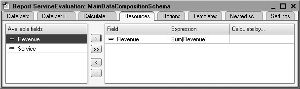
Fig. 13.28. Data Composition Schema Resources

Parameters

A user is normally interested in the data on economical activities over a specific period. This is why almost any report uses the parameters that define the beginning and the end of the report period.

Report parameters define the conditions for records to be included in the report. In the data composition schema the report parameters are defined on the Parameters tab (fig. 13.29).

You see three parameters on this tab: BeginOfPeriod, EndOfPeriod, and ProductType. You may be wondering why we have three parameters here while in the query we only specified one - ProductType?

The thing is that the data composition system analyses query text independently and in addition to the explicitly specified parameters (ProductType) makes it possible to customize parameters of virtual tables that participate in the query.

BeginOfPeriod and EndOfPeriod are such parameters. These are the two initial parameters of the virtual table named AccumulationRegister.Sales.Turnover that we used in the query in the left join.

If in the query wizard you highlight this table in the list of tables and click Virtual Table Parameters, a dialog will be displayed where you will see the BeginOfPeriod and EndOfPeriod parameters (fig. 13.30).

Fig. 13.30. Virtual table parameters

The first parameter transfers the beginning of the totals calculation period while the second one provides the end of such period. As a result the source will contain only turnovers calculated for the specified period.

We should always bear in mind that if we pass a date as one of these parameters (and that will be the case here), the date will also contain time, with precision down to one second.

Suppose that we know in advance that the user will not want to know the report results for the periods specified in seconds. In this case we should note two features.

First of all, we need to eliminate the need for the user to specify time when entering dates for the period a report should be generated for.

To do so, we will modify existing type definition for the BeginOfPeriod parameter.

Return to the Parameters tab of the data composition schema and doubleclick the cell Type for the BeginOfPeriod parameter.

Now click the selection button and in the bottom of the data type editor select Date for the Date Contents. Click OK (fig. 13.31).

Fig. 13.31. Editing date content

Another feature is that by default 00:00:00 is used as the time for a date. Hence if a user specifies a calculation period from 7/1/2010 to 7/14/2010, totals for the register will be calculated from the beginning of 7/1/2010 00:00:00 to the beginning of 7/14/2010 00:00:00. Hence the data for the 14^th day of the month other than those available at the beginning of the day will not be included in the report which may be confusing to the user.

In order to eliminate this situation, we will add another parameter where the user will enter the end date. And the value for the EndOfPeriod parameter we will calculate automatically so that it points to end of day for the userentered date.

This is why for the EndOfPeriod parameter we will check Availability Restriction. (fig. 13.32).

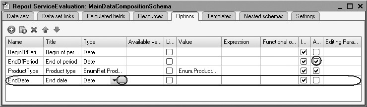
If it is left cleared, the parameter will be user-customizable. But if it is checked, the user will simply not see this parameter.

Next using the Add button in the command bar we will add a new parameter named EndDate (see fig. 13.32). The platform will automatically generate a title for this parameter - End Date. We will leave it unchanged.

Specify the type of the parameter value as Date. Same as for the Begin of Period specify the contents of the date as Date.

And for the BeginOfPeriod parameter create a title to be displayed to the user as Begin Date.

Note that by default the added parameter is available to the user (availability limitation is cleared in the column). This is fine with us.

Now switch to the EndOfPeriod parameter. For this parameter we have checked Availability Restriction because we intend to calculate the value for this parameter based on the value a user enters for the EndDate parameter.

In order to declare a formula to be used for calculation of the EndOfPeriod parameter value we will use expression language of the data composition system.

This language includes a function named EndOfPeriod() that enables us to get a date that corresponds to the end of some period, e.g. a specified day.

In the Expression cell enter the following expression for the EndOfPeriod parameter (listing 13.9).

Listing 13.9. Expression to calculate the value of the EndOfPeriod parameter

EndOfPeriod(&EndDate,"Day")

NOTE

For detailed description of the expression language available in the data composition system, see the built-in help under Help Help Contents

1C:Enterprise Script Common Objects Data Composition System Expression Language of the Data Composition System.

Once we are done with the above steps, the composition parameters will look as shown on the figure 13.33.

Finally, we will set up the ProductType parameter.

Since the report should display the revenue generated by sales of services only, the value of the ProductType parameter should not be edited by the user. It should be specified directly in the composition schema as Enumeration.ProductType.Service.

Availability restriction has been checked by default for the ProductType automatically so we only need to specify the required value of the ProductTypes enumeration in the cell Value that corresponds to the ProductType parameter.

Now use the selection button and select the value from the list of product types enumeration - Service (fig. 13.34).

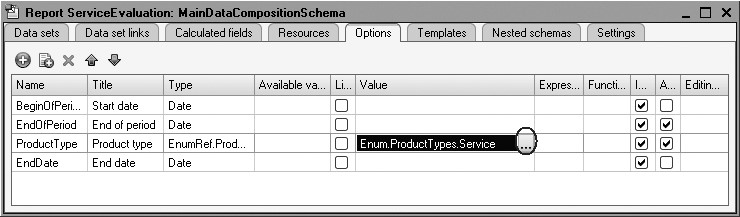
Fig. 13.34. Specifying the value for ProductType parameter

Settings

Now proceed to generating report structure.

On the Settings tab add a grouping without specifying the field to group by again.

On the Selected Fields tab specify the fields Service and Revenue

(fig. 13.35).

Fig. 13.35. Report structure for ServiceEvaluation

Now go to the Other Settings tab and enter a title for the report as Service Evaluation (fig. 13.36).

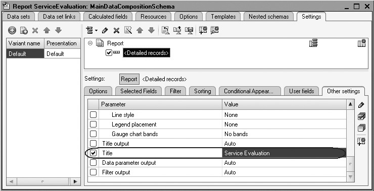
Fig. 13.36. Entering report title

NOTE

When we modify settings that require selection of some value, doubleclick the Value field to highlight it, click the selection button and select the required option from the list. Use flag for the value will appear automatically. You can also check and uncheck it manually.

Quick Custom Settings

Finally, we should make it possible for the user to define the report period before generating the report. This means that the Begin Date and End Date parameters should be included into the list of custom settings.

And since it is almost always required to specify a report period, these settings should be available directly in the report form.

On the Parameters tab we see the parameters that we have made editable for the user, i.e. cleared Availability Restriction (fig. 13.37).

Highlight the parameters one by one and click Properties of custom settings item button in the lower right corner of the settings window.

Check Include in custom settings and leave the default value Quick Access for Edit Mode property.

Note that Include in custom settings checkbox means that this specific setting will be available to a user in a new window (2) when the user clicks Settings (i.e. this is the setting that is available to the user but not for a very frequent use, fig. 13.38).

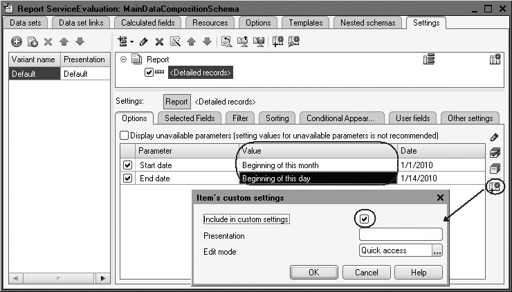
Fig. 13.37. Defining custom settings

Fig. 13.38. Quick (1) and ordinary (2) custom settings

And Quick Access value for the edit mode means that this setting will also be automatically displayed directly in the report form (1). This is a quick custom setting - the setting that a user will need frequently or almost every time the report is initiated. This is why this setting is always visible.

Besides, to further improve user interface, we will define for the parameters Begin date and End date initial values as Beginning of this month and Beginning of this day (see fig. 13.37).

This means that when the report is executed, the begin and end dates of the report period will change dynamically so that the report displays data from the beginning of the current month up to the current day and the user will probably not even need to modify them manually.

Finally, we will define the subsystems where our report will be displayed.

Close the data composition schema wizard and in the editor of the ServiceEvaluation Report configuration object navigate to the Subsystems tab.

Check the following subsystems in the list of configuration subsystems: Rendering Services and Accounting.

So a link to our report will be automatically added to the action panel of these subsystems (fig. 13.39).

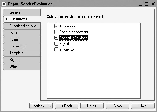
Fig. 13.39. Subsystems where report is displayed

In the 1C:Enterprise Mode

Launch 1C:Enterprise in the debugging mode and see how the report works.

In the 1C:Enterprise window that opens you see that the action panel of the Rendering Services and Accounting sections now has a command to execute the report named Service Evaluation in the group of commands for reports execution (fig. 13.40).

Execute this command.

This will open an automatically generated report form.

In the report window you see the parameters that define the report period. But by default the period is already specified: from the beginning of the month to the current day. If required, you can modify this period using the calendar button.

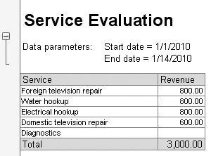
Click Generate. The result will look as follows (fig. 13.41):

Fig. 13.41. Report execution results

This means that revenue generated by all the three documents named Services Rendered we have created has been included in the report.

Note that the header of the report results window displays the title we have entered along with the parameters that specify the report period.

Now change the end date to be 1/13/2010. You can see that the data of July 13 from the document Services Rendered No. 1 (the last date of the report period) is included in the report (fig. 13.42).

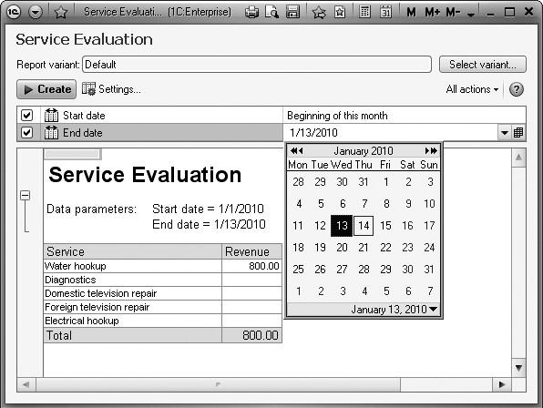
Note that since in the data query for the report the products table is connected to the sales register table using left join, the services that are not accompanied by any data of sales are still displayed in the report.

Settings in the Designer and Settings in the 1C:Enterprise Mode

Now using this report as an example we will demonstrate how other report settings can be created and used: Conditional Appearance and Filter.

In the process of creating these settings, we will perform some actions in the Designer and then switch to the 1C:Enterprise mode to review the effect.

But actually all the actions that we will perform in the Designer mode can be accessed in the 1C:Enterprise mode as well using the command All Actions4Change Variant. The difference is as follows.

The settings we will apply in the Designer are referred to as default settings and are saved in the data composition schema itself, i.e. will become a part of the configuration. This means that any configuration user will see the report exactly as we have set it up in the Designer.

All such settings can be applied in the 1C:Enterprise mode as well but these settings will not be a part of the configuration and will only be accessible to one specific user of a specific infobase.

NOTE

A configuration may have a mechanism developed that enables exchange of settings among various users. But this is not a simple job and we will not discuss it in this book - just know that it is possible.

The feature of editing report variant in the 1C:Enterprise mode is not intended for a regular user (quick settings and custom settings are sufficient for such users). Instead this feature is intended for a developer working on implementation, for an administrator or a very experienced user.

It is obvious that the settings applied in the 1C:Enterprise mode will override default settings. If a user has changed the report in a manner that it is totally different from the original version, you can always return to default settings using All Actions4Standard Settings.

Since right now we want to customize the report for all the users who will access this report, we will do it in the Designer.

But if one day the chief accountant asks you to make the report look better, you will be able to redo everything without modifying the configuration and right when she is watching.

Conditional Appearance

When it comes to the Service Evaluation report, it is convenient to highlight some report records with color for the records that contain services with the lowest or the highest revenues or based on some other condition.

In the Designer Mode

To do so, return to the Designer and open data composition schema on the Settings tab.

In the bottom of the window go to the Conditional Appearance tab and click Add in the upper right corner of the settings window (fig. 13.43).

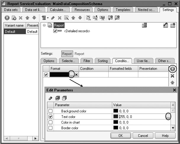
First we will define Appearance, i.e. exactly how the required fields should be highlighted.

Click the selection button in the Appearance field and choose red text color.

Click OK.

Next define the Condition for the appearance to be applied (for the text to turn red in our situation).

Click the selection button in the Condition field and in the window that opens add a New Item for the filter.

Every filter item specifies one condition. Multiple conditions may exist (fig. 13.44).

To do so, click the Add button and specify the following values: for the Left Value column - field Revenue, for the Comparison Type column - Less Than, and for the Right Value column - 700.

Click OK.

This means that when the Revenue field has a value under 700, red text color will be applied to something.

Now we will define this very something by declaring the list of formatted fields.

If you want to highlight the entire row of the report, this list may be left blank. Alternatively you can click the selection button in the Formatted Fields and in the window that opens select the fields Service and Revenue using the Add button (fig. 13.45).

In our situation we could skip this step because Service and Revenue are actually the only fields of the report.

Click OK.

Finally we will enter a Presentation for the conditional appearance:

Unpopular Service (fig. 13.46).

Unpopular Service is what a user will see in the available settings. So instead of a scary line reading "Revenue under 700...", the user will see a meaningful expression that is entered in the Presentation field.

Now we have defined a conditional appearance for the report where all the services with a revenue under 700 rubles will be considered as unpopular services and will be highlighted by red text color.

Now we will add this condition into custom settings.

Click Properties of custom settings item located in the lower right window of the settings window (see fig. 13.46).

Check Include in custom settings and select Normal for Edit Mode.

So you have included the created conditional appearance into ordinary custom settings. Unlike quick settings, custom settings are not located in the report form and can only be accessed in a new window by clicking the Setup button. This arrangement is due to the fact that such custom settings are used much less frequently than, for example, report period settings.

In the 1C:Enterprise Mode

Switch to the 1C:Enterprise mode. Open the report.

Specify End Date for the report period as Beginning of this day and click Generate (fig. 13.47).

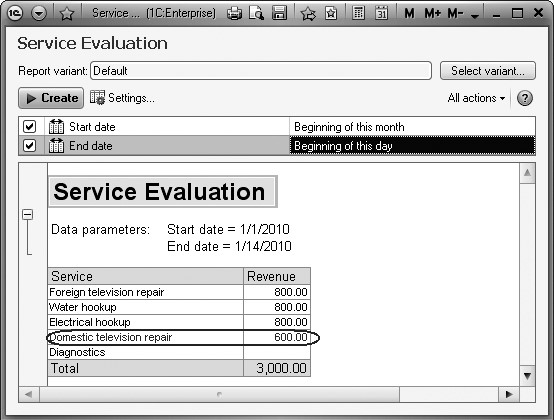
You see that the service amounts under 700 rubles are now highlighted in red.

Click the Setup button.

You will see the window of custom report settings that contains the report period parameters and setting for the Unpopular Service conditional appearance.

You can clear this setting, click Finish editing (fig. 13.48) and execute the report again.

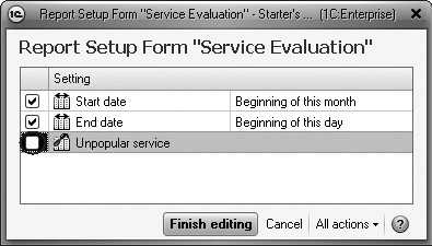
Color highlighting will disappear.

The Unpopular Service setting is not visible in the report form because for this setting we have selected Normal for edit mode instead of Quick Access.

But this conditional appearance setting is strictly defined and a user can only check or clear its use .

But to more experience users we can offer greater freedom in using settings, for example availability of defining report settings: filter, order, conditional appearance, etc.

Let us review it in the following example.

Custom Settings

In the Designer Mode

Return to the Designer.

On the Settings tab of the data composition schema you see all the settings of the report defined by the developer. Some of the settings can be provided to a user so that the user could create an arbitrary filter, conditional report appearance, etc.

To do so, click Properties of custom settings item located above in the command bar of the settings window (fig. 13.49).

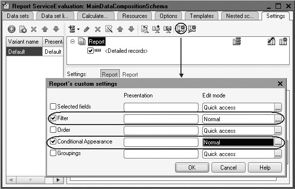
In the window that opens you can edit the assortment of custom settings for a report.

Select Use checkboxes for the settings Filter and Conditional Appearance and select Ordinary for the Edit Mode property.

So you have included settings for filter and conditional appearance into custom settings and made it possible for the users to edit them in a new window opened using the Setup button.

Filter

In the Designer Mode

Now we will create a filter setting in the report.

To do so, in the bottom of the setting form navigate to the Filter tab.

On the left you will see a list of the report fields available.

Expand the Service field and double-click the Parent field to move it to the list of filter conditions in the right pane of the window (fig. 13.50).

So we have made it possible to filter by groups of services that a user can define in the 1C:Enterprise mode.

In the 1C:Enterprise Mode

Open the report in the 1C:Enterprise mode and click Setup.

The window of custom report settings now has the settings Filter and Conditional Appearance that you have just checked (fig. 13.51).

In reality, here you see two conditional appearance settings.

The Unpopular Service setting has been predefined in the Designer. And now that you have added a setting for general conditional appearance, you have made it possible for a user to create any number of their own conditions for conditional appearance same as you have done it in the Designer. We will not do it right now but you can try it yourself.

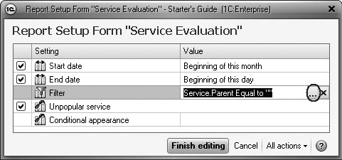
The next step will be defining a filter in the report so that it only includes the services related to washing machine installation.

To do so, click the selection button in the custom settings window in the Filter row (see fig. 13.51).

In the Edit Filter window that opens you can see the filter condition created earlier in the Designer.

The only thing you have to do is click the selection button in the Value row, expand the Services group and select the Washing Machines folder from the Products catalog (fig. 13.52).

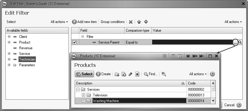
Click OK.

So we have defined a filter by the services that have the Washing Machines group of the Products catalog as their parents.

In the custom settings window click Finish editing and execute the report by clicking the Generate button (fig. 13.53).

You see that the report now only includes the services related to washing machine installation and the report header displays the information about this filter.

If you open the settings window, you can clear the filter setting by clicking the clear button or by creating another condition using the selection button in the Filter row (fig. 13.54).

Fig. 13.53. Report execution results

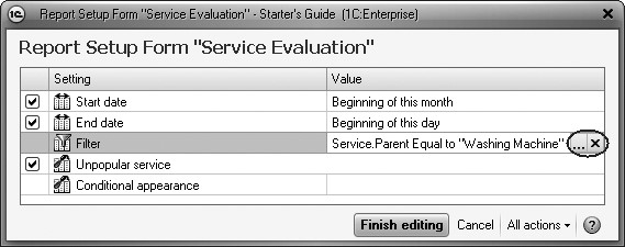
Fig. 13.54. Custom settings window

So if the user has enough skills, they will be able to define many settings as required.

If the user does not need to do so or does not have required skills, it will be better to specify the settings explicitly for the user to only enable or disable them.

In fact, often the report period or some other vital setting are enough and such settings should obviously be located directly in the report form.

Now we will return to the Designer and clear use for the filter setting.

We will need it in subsequent examples.

Display of Data for All the Days in the Selected Period

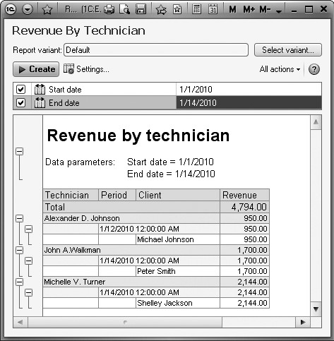
The next report we will add is named Revenue By Technician.

This report will contain information regarding the amount of revenue received at Jack of All Trades through the performance of each of its technicians, with a daily breakdown within a selected period and additional information concerning the clients to whom services were rendered on each of those days (fig. 13.55).

Using this report as example, we will demonstrate how to construct multilevel groupings in a query and how to search in all the days of the selected period.

We will demonstrate setup of individual items of the report structure and will also learn how to export data into a chart and create multiple report variants in the Designer.

In the Designer Mode

Add a new Report configuration object.

Enter RevenueByTech for the report name and run the data composition schema wizard.

Add a new Data Set - Query and open the query wizard.

For the query data source select the virtual table of the Sales.Turnover accumulation register.

Query for a Data Set

Virtual Table Parameters

Define one of the virtual table parameters: Periodicity.

To do so, go to the Tables field, highlight this table and click Virtual Table Parameters (fig. 13.56).

In the parameter window that opens define the value for Periodicity as Day (fig. 13.57).

Fig. 13.56. Modifying virtual table

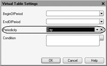
Fig. 13.57. Virtual table parameters parameters

Click OK.

Next select the following fields from the table (fig.13.58):

• SalesTurnover.Technician;
• SalesTurnover.Period;
• SalesTurnover.Client;
• SalesTurnover.SalesRevenue.

Now go to the Unions/Aliases tab and enter Revenue as the alias for the SalesTunover.SalesRevenue field (fig. 13.59).

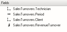
Fig. 13.58. Selected fields

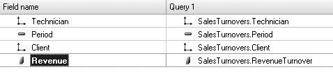
Fig. 13.59. Unions/Aliases

Analysis of Query Text

Click OK and review the query text generated by the wizard (listing 13.10).

Listing 13.10. Query Text

SELECT 
	SalesTurnovers.Technician, 
	SalesTurnovers.Period, 
	SalesTurnovers.Client, 
	SalesTurnovers.RevenueTurnover AS Revenue 
FROM 
	AccumulationRegister.Sales.Turnovers(,, Day, ) AS SalesTurnovers

In the query definition section note that the data source has a periodicity of selected data as Day (listing 13.11).

Listing 13.11. Defining Periodicity for a Virtual Table

FROM
	AccumulationRegister.Sales.Turnovers(,, Day, ) AS SalesTurnovers

This makes it possible for us to define the Period field among the selected fields.

Resources

Now proceed to editing of the data composition schema.

On the Resources tab click to make sure that the wizard has selected the only resource we have - revenue.

Parameters

On the Parameters execute the same actions we used when creating the previous report.

For the BeginOfPeriod define a title as Start Date. In the Type field select the date contents as Date.

Next add another parameter named EndDate and select Date for its type with Date as the date contents.

For the EndOfPeriod parameter define an expression (listing 13.12) and check the Availability Restriction field.

Listing 13.12. The expression to calculate the value of the EndOfPeriod parameter

EndOfPeriod(&EndDate,"Day")

Once we are done with the above steps, the data composition parameters will look as shown on the figure 13.60.

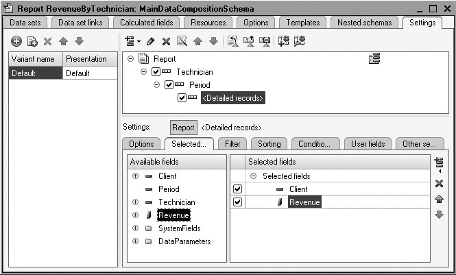
Settings

We will now create the report structure.

On the Settings tab create two nested groupings in succession:

n Top level - by the Technician field, n Nested - by the Period field.

To do so, first highlight the Report root item in the report structure, click Add in the command bar of the settings window, add a new grouping and select Technician as the field to group by (fig. 13.61).

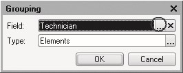
Fig. 13.61. Grouping field

Now add a nested grouping by the Period field to the Technician grouping.

To do so, highlight the Technician grouping, click Add, add a new grouping and select Period as the field to group by.

Now add another grouping nested to the Period grouping - Detailed Records (without selecting a field to group by).

To do so, highlight the Period grouping, click Add and add a new grouping without selecting a field to group by.

Next go to the Selected Fields tab and add Client and Revenue to the list of selected fields.

We are not selecting the fields Technician and Period because these fields are used to group data by so their values will be displayed automatically.

As a result of the actions above the report structure will look as follows (fig. 13.62):

Finally go to the Other Settings tab and modify the following parameters.

For the Grouping field placement select Separately and only in totals as the value.

By default grouping fields are located one under another vertically in a report (fig. 13.63).

Selecting Separately and only in totals as the value for this property means that every grouping will be located in a separate report area from left to right and its name will be displayed only in this grouping (fig. 13.64).

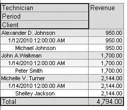
Fig. 13.63. Default vertical arrangement of grouping fields and totals

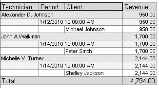
Fig. 13.64. Arrangement of grouping fields as Separately and Only in Totals

For the Vertical arrangement of overalls parameter select Beginning as the value.

By default totals are located in the end vertically (see fig. 13.63). Selecting this value for the property means that overalls will be displayed in the beginning prior to the grouping rows (fig. 13.65).

Fig. 13.65. Vertical arrangement of totals in the beginning

As a result of these actions other report settings will look as follows (fig. 13.66):

Fig. 13.66. Parameters of report display settings

Here we will also select Revenue By Technician as the value for Title.

Next specify that the parameters Begin Date and End Date will be included in the list of custom settings and these settings will be located directly in the report form, i.e. will serve as quick settings.

So before a report is actually generated, a user will be able to define a period for the report (fig. 13.67).

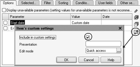
Fig. 13.67. Creating quick settings of report period

Finally, we will define the subsystems where our report will be displayed.

Close the data composition schema wizard and in the editor of the RevenueByTech Report configuration object navigate to the Subsystems tab.

Check the following subsystems in the list of configuration subsystems: Rendering Services and Payroll. So a link to our report will be automatically added to the action panel of these subsystems.

In the 1C:Enterprise Mode

Launch 1C:Enterprise in the debugging mode and see how the report works.

In the 1C:Enterprise window that opens you see that the action panel of the Rendering Services and Payroll sections now has a command to execute the report named Revenue By Technician in the group of commands for reports execution.

Execute this command.

Define 1/1/2010 to 1/14/2010 as the report period and generate the report (fig. 13.68).

Display of All Dates in a Selected Period

If you recall, at the beginning of the section we said that this report should provide a breakout for each day within a given period.

So far, our report only reflects those days that have non-zero records in the Sales accumulation register table.

To add further details in the report data, the data composition system makes it possible to specify period additions for groupings with a specified periodicity within the defined time period.

So we will now modify report settings so that the report includes every day of the specified period the report is generated for.

In the Designer Mode

Return to the Designer mode and further fine-tune the report structure.

Open data composition schema on the Settings tab.

Up to this point all the structure settings we executed applied to the entire report. But data composition system makes it possible to adjust every structure item independently as well.

CAUTION

When you work on report settings setup, you should see a button highlighted in the middle of the window under the report structure tree that corresponds to the setup mode. Report button for customization of the entire report or a button carrying a grouping name, e.g. Detailed Records, if such settings only apply to this grouping.

Now you will need to edit settings of the Period grouping.

To navigate to the settings of this particular grouping, in the report structure field point your cursor to this grouping and click Period in the command bar of the window.

The bottom of the window will display the settings available for this grouping.

Navigate to the Grouping Fields tab. For the Period field select Addition Type - Day (fig. 13.69).

In doing so, you specify that for this grouping the existing records with non-zero values of the resource will be complemented by the records for every day.

Next specify the period for such an addition to be executed.

In the fields of the row below you can enter the beginning and end dates for this period. But it is not enough for us to explicitly specify the dates because a user can generate a report for an arbitrary period. So we want this dates addition to be applied to the period selected by the user for the entire report instead of some fixed period.

For the report to work as required, double-click the Period Start Date field to enter edit mode, and click the clear button .

Next click the data type selection button to select the type of data displayed in this field.

Select Data Composition Field (fig. 13.70).

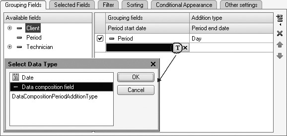
Fig. 13.71. Selecting data type

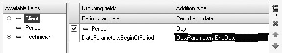
Click OK. Now click the selection button in the text box and in the selection window that opens check BeginOfPeriod (fig. 13.71). Click OK

Fig. 13.71. Field selection

In a similar manner specify for the second field that the period end date will be obtained from the EndDate parameter (fig. 13.72).

In the 1C:Enterprise Mode

Launch 1C:Enterprise in the debug mode and generate the Revenue By Technician report for the period from 1/10/2010 to 1/15/2010 (fig. 13.73).

Fig. 13.73. Report execution results

New Report Variant

For analysis of technicians' performance over a specific period, you may need to display the same information in another view that may be easier understandable.

For example, when your CEO makes payroll decisions, he may need to see a chart displaying the portion of every technician in the entire company's revenue over the period to understand who works better.

This is why we will now create another variant of the RevenueByTech report that will display the data as a chart.

Chart

A chart is intended to display various charts and diagrams in tables and forms.

Generally speaking, a chart consists of points, series and series values in points (fig. 13.74).

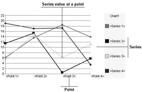
Fig. 13.74. Sample chart

As a rule, points are moments in time or objects for which we obtain the values of some characteristics, while series are those characteristics that we want to know values of. Chart values are located at intersections of series and points.

For example, a chart depicting monthly sales for types of products will consist of points (months), series (types of products), and values (sales revenues).

As a 1C:Enterprise script entity a chart has three areas that allow for management of chart appearance: plot area, header area, and legend area (fig. 13.75).

Fig. 13.75. Chart areas

A chart may be inserted into the report structure as an independent item. In the next variant of settings for RevenueByTech report we will use a chart in the settings structure of the data composition schema.

In the Designer Mode

Return to the Designer and open data composition schema on the

Settings tab.

The left pane of the window displays a list of report variants.

When report settings are first created, data composition system automatically creates a Default settings variant. We see this variant in the list for our report.

To add a new variant, click Add above the list. Enter a name for the variant: RevenueAmount (fig. 13.76).

We see that the report structure and all report settings have been cleared.

But they are not gone - instead they are simply invisible because they apply to the Default settings variant.

If a report has multiple variants, we can only see and edit the settings for the currently selected variant. And the remaining information of the data composition schema (resources, parameters, data sets) is leaved unchanged. The data for the report will be obtained using the very same database query. The only thing that is different is the settings that define how the report is displayed.

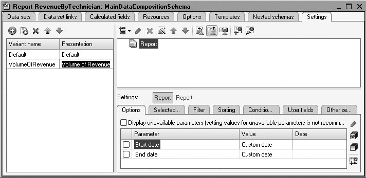
Fig. 13.76. Adding new settings variant

Now add a chart to the report structure. To do so, highlight the Report root item, open its context menu and add a chart (fig. 13.77).

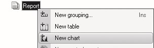
Fig. 13.77. Adding a Chart to Report Structure

Now highlight the Points branch and add a grouping by the Technician field to this branch.

Series of the chart should remain unchanged.

A gauge will be very convenient to show the share of every technician in the entire revenue amount. This is the chart we will use. For this chart type only points are enough so we are not specifying series.

One of the report resources is always used as a chart value. We only have one resource which is Revenue (the resource field is marked with a respective icon and is different from ordinary fields).

So you should now navigate to the Selected Fields tab, go to the level of entire report settings (by clicking the Report button) and select the field Revenue to be output to the report.

The report structure should look as follows (fig. 13.78).

Fig. 13.78. Report structure and chart settings

CAUTION

A chart should necessarily have a report resource. Otherwise it will result in an error.

On the Other Settings tab select Gauge as the chart type (fig. 13.79).

Scroll through the list of gauge properties and define gauge bands: Bad, Good, and Excellent (fig. 13.80).

Finally, we will include Begin Date and End Date as custom settings and select Quick Access for their Edit Mode.

CAUTION

For every report variant you need to specify the assortment of custom settings independently because every report variant has its own custom settings.

In the 1C:Enterprise Mode

Run 1C:Enterprise in the debugging mode and select Revenue By Technician in the action panel of the Payroll section.

In the report window that opens click Select Variant (fig. 13.81).

In the report variant window you now see two variants: Default variant and the Revenue Amount we have just created. Select this variant and click the Select button.

Define 1/1/2010 to 1/15/2010 as the report period and generate the report (fig. 13.82).

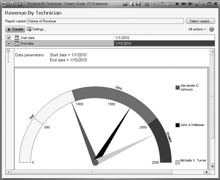
In the results you see exactly the same data as in the default report variant but displayed as a gauge. This chart makes it visually convenient to view the share of every technician in the entire revenue volume. Note that tooltips are displayed whenever the pointer is located over one of the chart's wedges.

But if you need to view the data for some technician with information regarding days and clients, it will be sufficient to select the Default report variant and reformat the report.

So, using Revenue By Technician report as an example, we have demonstrated how to create and use multiple report variants to better display information on performance of technicians.

Getting Current Values from a Periodic

Information Register

The next report is named Service List. It will contain information regarding the services provided by Jack of All Trades and their prices (fig. 13.83).

Using this report as an example, we will familiarize ourselves with how to get the latest values from a periodic information register and how to display hierarchical catalogs.

In the Designer Mode

Add a new Report configuration object.

Enter ServiceList for the report name and run the data composition schema wizard.

Add a new Data Set - Query and open the query wizard.

Query for a Data Set

As a data source for the query select an object (referential) table of the Products catalog and a virtual table of the Prices.SliceLast information register.

In order to avoid ambiguous names in the query, change the name of the Products table to ProductsCat.

To do so, highlight it in the Tables list, open its context menu and select Rename Table.

Virtual Table Parameters

Now open the dialog to enter parameters for the virtual table PricesSliceLast and specify that the period will be passed in the ReportDate parameter.

To do so, highlight this table in the Tables list and click Virtual Table Parameters (fig. 13.84).

Next select the following fields from the table (fig. 13.85):

• ProductsCat.Parent;
• ProductsCat.Ref;
• PricesSliceLast.Price.

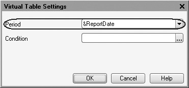
Fig. 13.84. Virtual table parameters

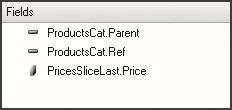
Fig. 13.85. Selected fields

Left Join of Tables

Switch to the Links tab and specify in the Link Condition that the value of Products dimension of the information register should be equal to the link to the Products catalog item.

Also clear All for the register table and select it for the catalog table. This is how we select left join as the link type for the catalog table (fig. 13.86).

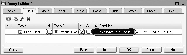
Fig. 13.86. Link of tables in a query

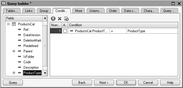
On the Conditions tab, enter the criteria for selecting items from the Products catalog - selected items should match the type of product that is passed in the Product Type parameter (fig. 13.87).

Field Aliases

On the Unions/Aliases tab, specify that the Parent field will have the alias ServiceGroup, and the Ref field will be referred to as Service (fig. 13.88).

Now you are done with creating the query so click OK.

Analysis of the Query Text

Now review the query text generated by the wizard (listing 13.13).

Listing 13.13. The query text

SELECT 
	ProductsCat.Parent AS ServiceGroup, 
	ProductsCat.Ref AS Service, 
	PricesSliceLast.Price 
FROM 
	Catalog.Products AS ProductsCat
	LEFT JOIN InformationRegister.Prices.SliceLast(&ReportDate, ) AS PricesSliceLast
		ON (PricesSliceLast.Products = ProductsCat.Ref)
WHERE 
	ProductsCat.ProductType = &ProductType

You are already familiar with virtually all the statements used in this query.

Proceed to editing of the data composition schema.

On the Resources tab click the button to select Price as the only available resource.

Parameters

On the Parameters tab define the value for the parameter named ProductType as Enumeration.ProductType.Service.

Besides, clear availability restriction for the ReportDate parameter.

In the Type field of this parameter select the date contents as Date.

For the Period parameter check availability restriction (fig. 13.89).

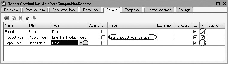
Fig. 13.89. Composition schema parameters

Settings

Now proceed to creating report structure. Go to the Settings tab, create a grouping by the field ServiceGroup and specify Hierarchy as the grouping type (fig. 13.90).

Fig. 13.90. Selecting grouping field and type

NOTE

Until now we have used No hierarchy as the default hierarchy type. The following hierarchy types are available for groupings in a report:

• No hierarchy - the grouping will only include non-hierarchical records.
• Hierarchy - the grouping will include both hierarchical and non-hierarchical records.
• Only hierarchy - the grouping will only include hierarchical (parent) records.

Create another grouping inside this one without specifying the field to group by. It will contain detailed report records.

Navigate to the Selected Fields tab and specify that the fields Service and Price will be included in the report (fig. 13.91).

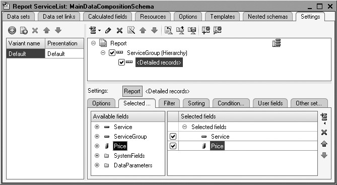
Fig. 13.91. Report structure and fields

Now customize report appearance on the Other Settings tab.

Since our report will simply serve as a list of available services where a user wants to see the prices for specific services, it makes no sense to display the values for the Price resource for every grouping and for the report in general. To disable display of overall totals in the report, select No as the value for Vertical arrangement of overalls (see fig. 13.93).

Now proceed to the settings for the specific grouping named ServiceGroup.

For the Totals Placement parameter of this grouping select No (fig. 13.92).

Fig. 13.92. Setup of overalls display for ServiceGroup grouping

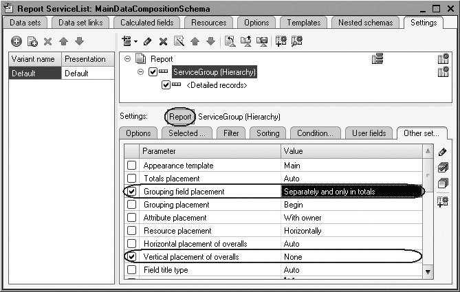
Fig. 13.93. Totals display settings for a global report

Now return to the settings applicable to the entire report.

For the Arrangement of Grouping Fields select Separately and Only in Totals (in this manner our report will be easier to understand) (fig. 13.93). Also enter Services List as the title for the report.

Finally, include Report Date parameter into custom settings and select Quick Access for its Edit Mode.

Also define the subsystems where our report will be displayed.

Close the data composition schema wizard and in the editor of the Services List Report configuration object navigate to the Subsystems tab.

Select the following subsystems in the list of configuration subsystems: Rendering Services and Accounting.

In the 1C:Enterprise Mode

Launch 1C:Enterprise in the debugging mode. First of all, open the Prices periodic register.

Add a new value for the service named Diagnostics: new price for the service as of 1/14/2010 - 350 (fig. 13.94). This will enable us to test the report.

Fig. 13.94. Adding a new record for diagnostics service in the Prices register

Now execute the Services List report as of 1/11/2010 (fig. 13.95).

Our report correctly reflects the price for Diagnostics service as of 1/11/2010, which was 200 rubles.

Run the report again, but this time with the date set to 1/14/2010 (fig. 13.96).

As you can see, the new price for Diagnostics is displayed as 350 rubles.

Fig. 13.95. Report execution results

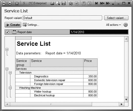
Fig. 13.96. Report execution results

This example has demonstrated how data composition system gets the latest values from a periodic information register and how to generate groups based on the catalog hierarchy.

Using Calculated Fields in a Report

The next report is named Client Evaluation and will visually demonstrate the return on services Jack of All Trades received from each client over its entire history (fig. 13.97).

Fig. 13.97. Report results

Using this report as an example, we will demonstrate use of a calculated field and display of the results as a pie chart or a column.

In the Designer Mode

Add a new Report configuration object.

Enter ClientEvaluation for the report name and run the data composition schema wizard.

Create a new Data Set - Query and open the query wizard.

Query for a Data Set

For the query data source select the virtual table of the Sales.Turnovers accumulation register.

Next select the following fields from the table (fig. 13.98):

• SalesTurnovers.Client;
• SalesTurnovers.RevenueTurnover;
• SalesTurnovers.CostTurnover.

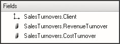
Fig. 13.98. Selected fields

On the Unions/Aliases tab, specify that the RevenueTurnover field will have the alias Revenue, and the CostTurnover field will be referred to as Cost.

Now you are done with creating the query so click OK.

There is nothing new or unclear in this query so we will not discuss it in details. Proceed to editing of the data composition schema.

Calculated Fields

On this stage we need to display a field in the report that is not available in the data set. In the previous reports we only used the fields defined in the data sets. Now that we need to display return on services per client, we also need an additional field calculated as revenue minus service cost.

To do so, the data composition system provides a feature of defining a calculated field.

Calculated fields are additional fields of the data composition schema with their values defined using some formula.

Go to the Calculated Fields tab of the data composition schema and click Add to add a calculated field.

Enter a name (Data Path) as Return. In the Expression column enter an expression for calculation of the field value (listing 13.14).

Listing 13.14. Expression for Calculation of Return Field Value

Revenue - Cost

A default title for the calculated field that will be displayed in the report header can be edited (fig. 13.99).

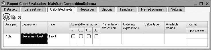
Fig. 13.99. Creating a calculated field

A calculated field can be added to report resources to calculate totals for groups and overalls using this field.

Resources

On the Resources tab click the button to select all the available report resources. As you can see, the calculated field named Profit has also been added to the list of resources (fig. 13.100).

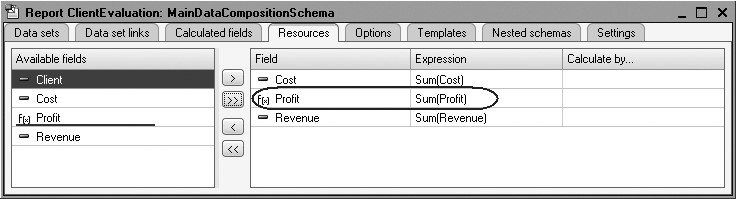
Fig. 13.100. Data composition schema resources

Settings

On the Settings tab add a chart to the report structure. To do so, click Add on the command bar of the settings window and add a chart (fig. 13.101).

Fig. 13.101. Adding a chart to report structure

Now highlight the Points branch and add a grouping by the Client field to this branch.

Series of the chart should remain unchanged.

The thing is that a pie chart will be very convenient to demonstrate client evaluation so we will use this type of chart. For this chart type only points are enough so we are not specifying series.

One of the report resources is always used as a chart value. Navigate to the Selected Fields tab and select the field Profit to be output to the report.

The report structure should look as follows (fig. 13.102).

Fig. 13.102. Report structure and chart settings

On the Other Settings tab select chart type as 3D Pie and enter a title for the report as Client Evaluation.

Finally, we will define the subsystems where our report will be displayed.

In the configuration object editor of the ClientEvaluation Report switch to the Subsystems tab.

Check the following subsystems in the list of configuration subsystems: Rendering Services and Accounting.

In the 1C:Enterprise Mode

Run 1C:Enterprise in the debugging mode and select Client Evaluation in the action panel of the Accounting section.

Click Generate.

You now see the data regarding return on services by client represented in a pie chart (fig. 13.103).

Now return to the Designer and change the chart type to 3D Column.

Regenerate the report (fig. 13.104).

Fig. 13.103. 3D pie chart

>

Fig. 13.104. 3D column

So we have now demonstrated how you can use various chart types to present report data visually.

Data Output to a Table

While we create a general purpose report, we will demonstrate how to output data to a table (fig. 13.105).

We will show how to make a report as generalist as possible to allow users to edit report structure and appearance in the 1C:Enterprise mode without using full report settings (i.e. using All Actions4Change Variant). For example, users might swap columns and rows of a table or change the data displayed in the table cells.

In the Designer Mode

Add a new Report configuration object.

Enter General for the report name and run the data composition schema wizard.

Create a new Data Set - Query and open the query wizard.

Query for a Data Set

For the query data source select the virtual table of the Sales.Turnover accumulation register.

Next select all the fields from the table (fig. 13.106).

Analysis of Query Text

Click OK and review the text generated by the query wizard (listing 13.15). Listing 13.15. The query text

SELECT
	SalesTurnovers.Product,
	SalesTurnovers.Client,
	SalesTurnovers.Technician,
	SalesTurnovers.QuantityTurnover,
	SalesTurnovers.RevenueTurnover,
	SalesTurnovers.CostTurnover
FROM
	AccumulationRegister.Sales.Turnovers AS SalesTurnovers

Resources

On the Resources tab click the button to select all the available report resources.

Settings

On the Settings tab add a table to the report structure.

To do so, click Add on the command bar of the settings window and add a table (fig. 13.107).

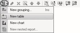
Fig. 13.107. Adding a table to report structure

We will not define rows and columns of the table here or a list of selected fields because we want to provide users with full freedom in their actions.

To do so, highlight the Table item in the report items structure and click Properties of custom settings item in the command bar of the settings window.

In the window that opens you can edit the assortment of custom settings for a table.

Select use for the settings Selected Fields, Row Groupings, and Column

Groupings and leave the default value Quick Access for their Edit Mode (fig. 13.108).

Fig. 13.108. Assortment of custom settings

So we have enabled a user to manually define the assortment of selected fields, groupings of rows and columns of the table directly in the report form prior to generating the report.

Finally, we will define the subsystems where our report will be displayed.

Close the data composition schema wizard and in the editor of the General Report configuration object navigate to the Subsystems tab.

Select Rendering Services subsystem in the configuration subsystem list.

In the 1C:Enterprise Mode

Run 1C:Enterprise in the debugging mode and select General in the action panel of the Rendering Services section.

If you now click Generate, we will see nothing in the results because the list of selected fields, groupings of rows and columns of the table is empty. Fill in these custom settings.

Click the selection button in the Selected Fields row and select the field named SalesRevenue from the list of available fields.

Click the selection button in the Rows row and add grouping by the field Product of the Hierarchy type to the table rows.

Click the selection button in the Columns row and add a grouping by the field Technician to the table rows.

Click Generate.

The report will look as follows (fig. 13.109).

Now add the field CostTurnover to the list of selected fields.

To the table rows we will add a grouping by the Client field instead of the Product field.

This will result in the following appearance of the report (fig. 13.110).

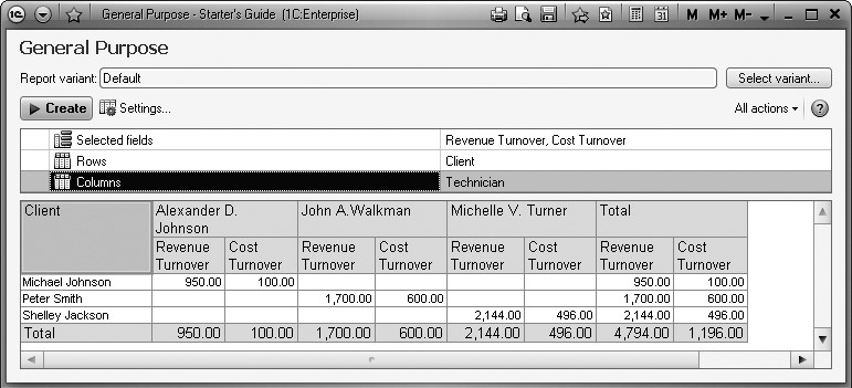
Now exclude CostTurnover from the list of selected fields.

In the table rows replace the previous grouping with a grouping by the Product field having HierarchyOnly as its type.

Add a grouping by the Client field to the table rows and locate it in the first place in the grouping list.

This will result in the following appearance of the report (fig. 13.111).

Fig. 13.111. Report results

So we have now used this report to offer a user an option to manually create a report for the Sales register.

Theory. Virtual Query Tables

As you now know, when creating a query, the platform gives us a number of virtual tables as data sources. "Virtual" is a good name for them, since these tables, in turn, are also the result of a query which the system generates at the moment when the corresponding block of code is executed.

For the most part, developers themselves can get all the same data that the system provides them in the form of virtual tables. However, the algorithm for getting that data will not be optimal for the following two reasons.

First, all of the virtual tables are parameterized. In other words, developers can define some parameters that will be used by the system in generating the query to create the virtual table.

We should point out here that when the developer specifies parameters for a virtual table, it does not always result in those values simply getting plugged into the query text. Depending on which virtual table parameters the developer specifies, the developer may generate DIFFERENT queries to get the same virtual table, but these queries will be optimized from the prospective of the parameters that were provided.

Second, the developer is not always able to access all the data available to the system. For example, when using virtual information register tables, the developer basically has access to all the information regarding register data that the system uses when it generates virtual table query.

But it is quite another matter when we deal with virtual tables of accumulation registers. Here the system dynamically generates the query depending not only on the parameters passed to it, but it also takes into account the period for the totals calculated in the register. When it does this, it uses data from those totals, which is simply not available for the developer to query.

Of course, the developer could also search through all the accumulation register records and get the same data provided by the system as a virtual table as a result. But obviously this query would be less efficient and will require more of the developer's time and effort.

Quiz

• What is the Query 1C:Enterprise script entity intended for?
• What is the data composition system intended for?
• What is the data composition schema intended for?
• What are the data composition settings intended for?
• What is the difference between actual tables and virtual tables?
• What sections does a query text consist of? Which sections are mandatory?
• What are basic syntax statements of query language?
• What data sources are used for a query?
• What is an alias in the query language?
• What are query parameters?
• What are virtual table parameters?
• What is the meaning of left join?
• How does one use query wizard?
• How does one select data from some period for a report?
• How does one order data in a report?
• How does one use data from multiple tables in a report?
• How does one use groupings in the report structure?
• How does one get the latest values from an information register?
• How does one display hierarchical data in a report?
• How does one manage display of totals for groupings and overalls?
• How does one create a report containing a chart?
• How does one use parameters in the data composition system?
• What are resources in the data composition system?
• What are calculated fields in the data composition system?
• How does one add all the days of a grouping by period to a report data?
• How does one create custom report settings?
• What is the difference between quick settings and ordinary custom settings?
• How does one define the assortment of custom settings for a report?
• How does one display data as a table?
• How does one make a report general-purpose?